Read and verify a bathymetry result

Looking for the regional map? Open the San Juan bathymetry atlas. This page remains the runnable synthetic companion.

Turn the offline demo into an inspectable table: check its provenance, identify the H3 support, and distinguish unavailable depth from observed zero variation. This example uses the installed production pipeline and its generated controls.

Synthetic inputs, real processing

The raster, datum and neighborhood are synthetic. The result demonstrates software behavior; it is not a San Juan survey, navigational chart, or audited regional release. No source acquisition is needed after installation.

1. Generate the example

Follow installation using Python 3.14, then run these commands in the same terminal with that environment activated:

export SEASCAPE_WORKSPACE="$(mktemp -d "${TMPDIR:-/tmp}/seascape-example.XXXXXX")"
seascape --workspace "$SEASCAPE_WORKSPACE" demo

The CLI prints Synthetic software acceptance: PASS (not a regional release) after all controls pass. It writes only within the workspace's .seascape/demo subtree. A fresh directory avoids overwriting any earlier experiment; see safe reruns for the explicit overwrite contract.

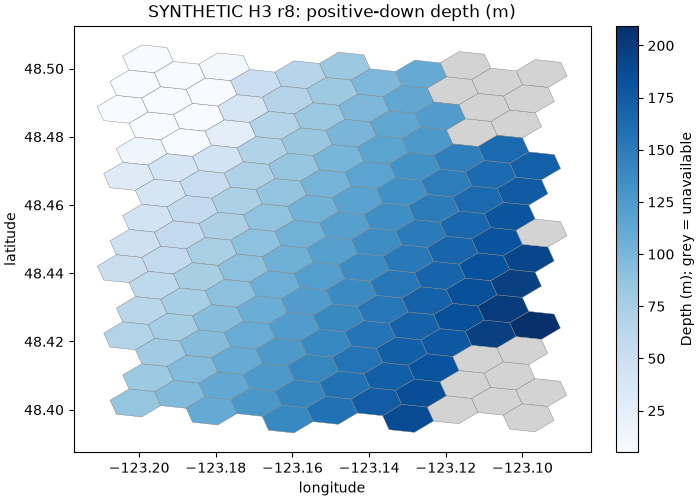
The illustration shows the demo's controlled gradient and missing coverage. Inspect your run's figures/input.png and figures/output.png beneath $SEASCAPE_WORKSPACE/.seascape/demo/ for the actual generated figures.

2. Read the table and verify its identity

Run this block in the same terminal. It reads the files produced above and checks the manifest's checksum before inspecting values. Pandas and H3 are runtime dependencies; Jupyter is not required.

python - <<'PY'
import json
import os
from pathlib import Path

import h3
import pandas as pd
from seascape.core.artifacts.checksums import checksum_path

root = Path(os.environ["SEASCAPE_WORKSPACE"]) / ".seascape/demo"
table_path = root / "output/BATHYMETRY.parquet"
report = json.loads((root / "report.json").read_text())
manifest = json.loads((root / "output/bathymetry_manifest.json").read_text())

assert report["status"] == "PASS"
assert report["checks"] and all(report["checks"].values())
assert report["metadata"]["synthetic"] is True
assert report["metadata"]["bathymetry_sign"] == "positive_down"
artifact = next(
    item for item in manifest["artifacts"]
    if item["path"] == "output/BATHYMETRY.parquet"
)
assert checksum_path(table_path) == artifact["checksum"]

table = pd.read_parquet(table_path)
assert table["H3_INDEX"].notna().all() and table["H3_INDEX"].is_unique
assert table["H3_INDEX"].map(h3.get_resolution).eq(8).all()
assert len(table) == report["row_count"] == artifact["row_count"]

valid = table["BATHYMETRY"].notna()
print(f"Rows: {len(table)}; columns: {len(table.columns)}")
print(f"Depth available: {valid.sum()}; unavailable: {(~valid).sum()}")
print("Source:", manifest["sources"][0]["name"])
print("Datum:", report["metadata"]["vertical_datum"])

by_cell = table.set_index("H3_INDEX")
controls = report["controls"]
flat = by_cell.loc[controls["flat"]]
assert abs(flat["BATHYMETRY"] - 5.0) <= 1e-6
assert flat["BATHYMETRY_STD"] == 0.0
assert flat["BATHYMETRY_FRAC_0_10_M"] == 1.0
assert flat["BATHYMETRY_FRAC_10_30_M"] == 0.0
for name in ("nodata", "outside", "sea_level"):
    assert pd.isna(by_cell.loc[controls[name], "BATHYMETRY"])

columns = ["BATHYMETRY", "BATHYMETRY_STD", "BATHYMETRY_PIXEL_COUNT"]
sample = by_cell.loc[list(controls.values()), columns].copy()
sample.index = list(controls)
print(sample.to_string(float_format=lambda value: f"{value:.3f}"))
PY

These assertions are executable checks: a mismatch stops the example rather than printing a successful interpretation. They complement the demo's 15 production acceptance checks; they do not rerun the scientific calculations independently. Use the toolkit's checksum helper: its SHA-256 identity includes the file name as well as the file bytes, so a raw file-only SHA-256 is not interchangeable.

3. Interpret the controls

The October 4, 2026 run of version 0.1.1 produced 153 rows and 33 columns: 135 rows had depth and 18 retained null depth. These are fixture counts, not a measure of regional coverage. Each row identifies one H3 R8 cell.

Control	Mean depth (m, positive down)	Standard deviation (m)	Valid marine pixels	Interpretation
Flat	5.000	0.000	18	Measured constant depth: zero variation is meaningful.
Gradient	120.851	5.049	18	Aggregation of the controlled synthetic slope.
Nodata	null	null	null	The source provides no usable depth here.
Outside	null	null	null	The support cell lies outside the raster.
Sea level	null	null	null	The existing marine mask excludes exact zero elevation.

Do not fill these nulls with zero: that would invent shallow-water observations. Likewise, a zero [10, 30) m fraction on the flat 5 m patch means none of its valid marine pixels fall in that band; it does not mean missing coverage.

BATHYMETRY is a mean of valid source pixel centers assigned to the cell, not a survey of every point inside its polygon. Pixel count supplies sampling context, not a complete uncertainty estimate. Distance-to-isobath columns have companion DISTANCE_TO_ISOBATH_*_STATUS fields: inspect them before interpreting null distances. The demo's H3 neighborhood is synthetic and does not establish actual coastal passability.

4. Choose the next step

• Inspect the full demo contract for sign, depth-band, gradient and checksum checks and their tolerances.
• Use the validation notebook for a notebook view of the same production API.
• Prepare bounded real-data inputs when you have reviewed sources and coverage.
• For an already audited regional release, use the release-backed product API. This demo has a family manifest, but does not create a canonical release for that resolver.